Semimetal-to-Mott-insulator transition

This notebook uses pyALF to simulate the repulsive Hubbard model on the honeycomb lattice at half filling. We vary the interaction strength and measure antiferromagnetic spin correlations as a function of system size. The aim is to connect the simulation workflow to the physics of the semimetal-to-Mott-insulator transition.

4.2.1Motivation and model¶

In a Dirac semimetal the valence and conduction bands touch at two isolated points, $\mathbf K$ and $\mathbf K'$ , at the Fermi energy. Near either point, the single-particle dispersion is of the form $\epsilon_{\mathbf q, \pm} \simeq \pm \hbar v_F|\mathbf q|$ , where $\mathbf q$ is measured from the Dirac point. The low-energy excitations behave as massless Dirac fermions: they are gapless, but their density of states vanishes at the Fermi energy. Weak short-range interactions therefore do not immediately destabilise this phase. On the other hand, a Mott insulator has an interaction-induced charge gap, which, due to strong electronic repulsion, the electrons localise. In the Hubbard model, strong on-site repulsion suppresses double occupancy and charge motion, leaving local magnetic moments. Magnetic order is not required for Mott insulation in general. On a bipartite lattice, such as the honeycomb lattice studied here, antiferromagnetic Néel order is developed, with opposite spin orientations on its two sublattices.

The Hamiltonian we study is given by:

\hat H = -t \sum_{\langle i,j\rangle,\sigma} (\hat c^\dagger_{i, \sigma} \hat c_{j, \sigma} + \mathrm{h.c.} ) + \frac{U}{2} \sum_i \left(\sum_\sigma \left(\hat n_{i,\sigma} - \frac12 \right) \right)^2

(1)

Here $\{\hat c_{i,\sigma}, \hat c^\dagger_{j, \sigma^\prime}\} = \delta_{i,j} \delta_{\sigma, \sigma^\prime}$ are fermionic operators which create a fermion in a Wannier wave function localised around a lattice site with position $\vec{r}_i$ with spin $\sigma = \uparrow, \downarrow$ . Furthermore, $t$ is the nearest-neighbour hopping, $U > 0$ is the on-site repulsion, and $\hat n_{i, \sigma}=\hat c^\dagger_{i, \sigma}\hat c_{i\sigma}$ . Owing to particle-hole symmetry, the system is at half-filling. The energy scale is set by the hopping parameter, which we set to unit $t = 1$ .

Increasing $U/t$ drives a quantum phase transition at a finite critical interaction: Néel order develops and the Dirac fermions become gapped. In the effective Dirac description, the ordered fermion bilinear acts as a mass term, giving a spectrum of the form $\epsilon_{\mathbf q, \pm} = \pm\sqrt{(\hbar v_F|\mathbf q|)^2+ m^2}$ , where $m$ is the mass gap. This connects the transition to dynamical mass generation in high-energy physics: interactions generate a condensate and a fermion mass, as in the Gross–Neveu model Gross and Neveu, 1974. The continuous transition belongs to the Gross–Neveu–Heisenberg universality class in $2+1$ dimensions, described by Dirac fermions coupled to a critical three-component Néel order parameter, as in the Gross–Neveu–Yukawa formulation. Other order-parameter symmetries give other Gross–Neveu classes; a two-component order parameter can give Gross–Neveu–XY criticality. The universality class also depends on the number of fermion flavours. Deep in the insulating regime, virtual hopping produces an antiferromagnetic exchange $J\simeq 4t^2/U$ between local moments. Large-scale studies find a direct, continuous zero-temperature transition near $U_c/t\approx 3.8$ , associated with Gross–Neveu–Heisenberg criticality, see Wang et al., 2026.

Although in an experimental setting we cannot change $U$ , we can effectively change $t$ in moiré materials. Twist angle, pressure and electric fields can tune moiré bandwidths and interaction effects. Transport measurements have revealed a continuous metal-to-Mott-insulator transition in semiconductor moiré superlattices (Li et al., 2021) and a bandwidth-tuned Mott transition in twisted WSe $_2$ (Xia et al., 2026). Complementary probes resolve the insulating state: infrared photocurrent spectroscopy detects excitations across an emerging Mott gap in trilayer graphene/hBN (Yang et al., 2022), while combined transport, compressibility and magnetic circular dichroism distinguish correlated insulating phases in MoTe $_2$ /WSe $_2$ (Chang et al., 2026). For Dirac transitions specifically, theory and numerics predicts Gross–Neveu–XY criticality between a semimetal and a Kramers intervalley-coherent insulator in twisted bilayer graphene (Biedermann and Janssen, 2025; Hawashin et al., 2025; Huang et al., 2025). Twisted double bilayer transition-metal dichalcogenides offer a proposed semimetal-to-antiferromagnetic-insulator transition in the Gross–Neveu–Heisenberg class, although heterostrain can change the lowest-temperature critical behaviour (Biedermann and Janssen, 2026). These proposals motivate combined gap, order-parameter and critical-scaling measurements; the observed Mott transitions above do not by themselves establish Gross–Neveu universality.

4.2.2Import the tools¶

Simulation prepares and runs ALF, while ALF_source manages its source directory. We use load_res to collect analysed observables, Lattice to locate a momentum in ALF’s lattice convention, and NumPy, pandas, and Matplotlib to organise and plot the results. Run the notebook from top to bottom after completing the installation steps.

import matplotlib.pyplot as plt  # Plotting library
import numpy as np  # Numerical libary
from py_alf import ALF_source, Simulation, Lattice
from py_alf.ana import load_res  # Function for loading analysis results
# from py_alf.analysis import analysis  # Analysis function
from py_alf.utils import find_sim_dirs  # Function for finding QMC bins

from pathlib import Path
import pandas as pd
from collections import defaultdict

4.2.3Set the ALF source directory¶

ALF_source locates the ALF source checkout, downloading it if necessary, and selects the requested branch. The resulting alf_src object is shared by the compilation and simulation steps. Here we use master; for a reproducible study, also record the ALF and pyALF versions used.

alf_src = ALF_source(branch='master')

4.2.4Compile ALF¶

Create a Simulation object for the Hubbard Hamiltonian and compile the executable once. This step builds ALF but does not perform a Monte Carlo run. The same executable can then be reused for all lattice sizes and interaction strengths in the scan. Compilation requires the Fortran compiler and numerical libraries described in the installation section.

compile_sim = Simulation(alf_src=alf_src, ham_name='Hubbard',sim_dict={}) #sim_dict is used to choose parameters.
compile_sim.compile()

Checking out branch master
Your branch is up to date with 'origin/master'.

Already on 'master'

Compiling ALF... 
Cleaning up Prog/
Cleaning up Libraries/
Cleaning up Analysis/
Compiling Libraries

entanglement_mod.F90:35:2:

   35 | #warning "You are compiling entanglement without MPI. No Renyi entropy results possible, all other observables still work!"
      |  1~~~~~~
Warning: #warning "You are compiling entanglement without MPI. No Renyi entropy results possible, all other observables still work!" [-Wcpp]
ar: creating archive modules_90.a
ar: creating archive libqrref.a

Compiling Analysis
Compiling Program
Compiling program modules
Parsing Hamiltonian parameters
filenames: Hamiltonians/Hamiltonian_Kondo_smod.F90 Hamiltonians/Hamiltonian_Kondo_read_write_parameters.F90
filenames: Hamiltonians/Hamiltonian_Hubbard_smod.F90 Hamiltonians/Hamiltonian_Hubbard_read_write_parameters.F90
filenames: Hamiltonians/Hamiltonian_Hubbard_Plain_Vanilla_smod.F90 Hamiltonians/Hamiltonian_Hubbard_Plain_Vanilla_read_write_parameters.F90
filenames: Hamiltonians/Hamiltonian_tV_smod.F90 Hamiltonians/Hamiltonian_tV_read_write_parameters.F90
filenames: Hamiltonians/Hamiltonian_LRC_smod.F90 Hamiltonians/Hamiltonian_LRC_read_write_parameters.F90
filenames: Hamiltonians/Hamiltonian_Z2_Matter_smod.F90 Hamiltonians/Hamiltonian_Z2_Matter_read_write_parameters.F90
filenames: Hamiltonians/Hamiltonian_Spin_Peierls_smod.F90 Hamiltonians/Hamiltonian_Spin_Peierls_read_write_parameters.F90
Link program
Done.

4.2.5Run the simulations¶

We scan $U/t=1,2,\ldots,7$ on periodic honeycomb lattices with $L=3,6,9$ . Each unit cell contains two sites, labelled $A$ and $B$ , so the number of unit cells is $N=L^2$ and the number of sites is $N_s=2L^2$ : 18, 72 and 162 sites, respectively.

The main parameters are:

Parameter	Meaning in this example
`Lattice_type`, `L1`, `L2`	Honeycomb geometry with $L\times L$ unit cells.
`ham_U`, `ham_chem`	Repulsive interaction $U>0$ and half filling at zero chemical potential.
`Beta`	Inverse temperature $\beta=1/T$ ; we choose $\beta t=L$ , so larger lattices are also colder.
`NBin`, `Nsweep`	Ten measurement bins with ten Monte Carlo sweeps per bin, intended for a short demonstration.
`Mz=False`	A Hubbard–Stratonovich transformation coupling the auxiliary field to the density and preserving spin-rotation symmetry for each field configuration.
`N_SUN=2`, `N_FL=1`	The two physical spin states are represented as two colours sharing one fermion flavour.
`Checkerboard`, `Symm`	A symmetric checkerboard decomposition of imaginary-time evolution. The remaining finite-time-step error must still be checked.
`Ltau=0`	Measure equal-time observables only; time-displaced correlations are unnecessary for the plot below.

The choice $\beta\propto L$ is motivated by the dynamical exponent $z=1$ at this quantum critical point. It fixes the space-time aspect ratio, but does not by itself establish ground-state convergence. The time step is not specified in the dictionary; the current ALF defaults give $\Delta\tau=0.1$ .

For each $(L,U)$ , sim.run() performs the simulation and sim.analysis() computes observable means and statistical errors. Each parameter set has its own directory. The directory prefix Attractive_Hubbard is only a name: the positive ham_U values here specify the repulsive model.

LAT_SIZES = [3,6,9]
U_VALS = [i for i in np.arange(1.0, 8.0, 1.0)]

for U in U_VALS:
    for L in LAT_SIZES:
        sim = Simulation(
                    alf_src, 'Hubbard',
                    {
                        ### Choice of Predefined Model###
                        'Model': 'Hubbard',
                        
                        ###Definition of the Lattice###
                        'Lattice_type': 'Honeycomb',
                        'L1': L,
                        'L2': L,
                        
                        #--- Model parameters ---#
                        'Beta': L,
                        'ham_chem': 0.0,
                        'ham_U': U,
                        #--- Simulation parameters --- #
                        'Nsweep': 10,
                        'NBin': 10,
                        'Mz': False, #Choice of HS-Transformation (Exclusive for Hubbard-type interactions); ALF-DOC: 8.3.2 M_Z-Hubbard interaction
                        'Checkerboard': True, #ALF-DOC: 2.3. The Trotter error and checkerboard decomposition
                        'Symm': True, #Symmetric Trotter decomposition; ALF-DOC: 2.3. The Trotter error and checkerboard decomposition

                        ###ALF Internal Flags###
                        'N_SUN': 2, #
                        'N_FL': 1, # 
                        'Ltau': 0, #Speed up simulation by not calculating time-displaced observables, which take more time to compute.
                    },
                    machine='GNU',
                    sim_dir=f'MOTT/Attractive_Hubbard_L{L}_U_{U}'
                )
        sim.run()
        sim.analysis()
print('All simulations and analyses complete.')

Prepare directory "/Users/luis/Documents/_WORK/CONFERENCES/ALF_WORKSHOP_26/ALF_Tutorial/jupyterbook/source/04-nice-physics/ALF_data/MOTT/Attractive_Hubbard_L3_U_1.0" for Monte Carlo run.
Create new directory.
Run /Users/luis/Documents/_WORK/CONFERENCES/ALF_WORKSHOP_26/ALF_Tutorial/jupyterbook/source/04-nice-physics/ALF/Prog/ALF.out
 ALF Copyright (C) 2016 - 2022 The ALF project contributors
 This Program comes with ABSOLUTELY NO WARRANTY; for details see license.GPL
 This is free software, and you are welcome to redistribute it under certain conditions.
 No initial configuration
### Analyzing /Users/luis/Documents/_WORK/CONFERENCES/ALF_WORKSHOP_26/ALF_Tutorial/jupyterbook/source/04-nice-physics/ALF_data/MOTT/Attractive_Hubbard_L3_U_1.0 ###
/Users/luis/Documents/_WORK/CONFERENCES/ALF_WORKSHOP_26/ALF_Tutorial/jupyterbook/source/04-nice-physics
Scalar observables:
Ener_scal
Kin_scal
Part_scal
Pot_scal
Histogram observables:
Equal time observables:
Den_eq
Green_eq
SpinZ_eq
Time displaced observables:
Prepare directory "/Users/luis/Documents/_WORK/CONFERENCES/ALF_WORKSHOP_26/ALF_Tutorial/jupyterbook/source/04-nice-physics/ALF_data/MOTT/Attractive_Hubbard_L6_U_1.0" for Monte Carlo run.
Create new directory.
Run /Users/luis/Documents/_WORK/CONFERENCES/ALF_WORKSHOP_26/ALF_Tutorial/jupyterbook/source/04-nice-physics/ALF/Prog/ALF.out
 ALF Copyright (C) 2016 - 2022 The ALF project contributors
 This Program comes with ABSOLUTELY NO WARRANTY; for details see license.GPL
 This is free software, and you are welcome to redistribute it under certain conditions.
 No initial configuration
### Analyzing /Users/luis/Documents/_WORK/CONFERENCES/ALF_WORKSHOP_26/ALF_Tutorial/jupyterbook/source/04-nice-physics/ALF_data/MOTT/Attractive_Hubbard_L6_U_1.0 ###
/Users/luis/Documents/_WORK/CONFERENCES/ALF_WORKSHOP_26/ALF_Tutorial/jupyterbook/source/04-nice-physics
Scalar observables:
Ener_scal
Kin_scal
Part_scal
Pot_scal
Histogram observables:
Equal time observables:
Den_eq
Green_eq
SpinZ_eq
Time displaced observables:
Prepare directory "/Users/luis/Documents/_WORK/CONFERENCES/ALF_WORKSHOP_26/ALF_Tutorial/jupyterbook/source/04-nice-physics/ALF_data/MOTT/Attractive_Hubbard_L9_U_1.0" for Monte Carlo run.
Create new directory.
Run /Users/luis/Documents/_WORK/CONFERENCES/ALF_WORKSHOP_26/ALF_Tutorial/jupyterbook/source/04-nice-physics/ALF/Prog/ALF.out
 ALF Copyright (C) 2016 - 2022 The ALF project contributors
 This Program comes with ABSOLUTELY NO WARRANTY; for details see license.GPL
 This is free software, and you are welcome to redistribute it under certain conditions.
 No initial configuration
### Analyzing /Users/luis/Documents/_WORK/CONFERENCES/ALF_WORKSHOP_26/ALF_Tutorial/jupyterbook/source/04-nice-physics/ALF_data/MOTT/Attractive_Hubbard_L9_U_1.0 ###
/Users/luis/Documents/_WORK/CONFERENCES/ALF_WORKSHOP_26/ALF_Tutorial/jupyterbook/source/04-nice-physics
Scalar observables:
Ener_scal
Kin_scal
Part_scal
Pot_scal
Histogram observables:
Equal time observables:
Den_eq
Green_eq
SpinZ_eq
Time displaced observables:
Prepare directory "/Users/luis/Documents/_WORK/CONFERENCES/ALF_WORKSHOP_26/ALF_Tutorial/jupyterbook/source/04-nice-physics/ALF_data/MOTT/Attractive_Hubbard_L3_U_2.0" for Monte Carlo run.
Create new directory.
Run /Users/luis/Documents/_WORK/CONFERENCES/ALF_WORKSHOP_26/ALF_Tutorial/jupyterbook/source/04-nice-physics/ALF/Prog/ALF.out
 ALF Copyright (C) 2016 - 2022 The ALF project contributors
 This Program comes with ABSOLUTELY NO WARRANTY; for details see license.GPL
 This is free software, and you are welcome to redistribute it under certain conditions.
 No initial configuration
### Analyzing /Users/luis/Documents/_WORK/CONFERENCES/ALF_WORKSHOP_26/ALF_Tutorial/jupyterbook/source/04-nice-physics/ALF_data/MOTT/Attractive_Hubbard_L3_U_2.0 ###
/Users/luis/Documents/_WORK/CONFERENCES/ALF_WORKSHOP_26/ALF_Tutorial/jupyterbook/source/04-nice-physics
Scalar observables:
Ener_scal
Kin_scal
Part_scal
Pot_scal
Histogram observables:
Equal time observables:
Den_eq
Green_eq
SpinZ_eq
Time displaced observables:
Prepare directory "/Users/luis/Documents/_WORK/CONFERENCES/ALF_WORKSHOP_26/ALF_Tutorial/jupyterbook/source/04-nice-physics/ALF_data/MOTT/Attractive_Hubbard_L6_U_2.0" for Monte Carlo run.
Create new directory.
Run /Users/luis/Documents/_WORK/CONFERENCES/ALF_WORKSHOP_26/ALF_Tutorial/jupyterbook/source/04-nice-physics/ALF/Prog/ALF.out
 ALF Copyright (C) 2016 - 2022 The ALF project contributors
 This Program comes with ABSOLUTELY NO WARRANTY; for details see license.GPL
 This is free software, and you are welcome to redistribute it under certain conditions.
 No initial configuration
### Analyzing /Users/luis/Documents/_WORK/CONFERENCES/ALF_WORKSHOP_26/ALF_Tutorial/jupyterbook/source/04-nice-physics/ALF_data/MOTT/Attractive_Hubbard_L6_U_2.0 ###
/Users/luis/Documents/_WORK/CONFERENCES/ALF_WORKSHOP_26/ALF_Tutorial/jupyterbook/source/04-nice-physics
Scalar observables:
Ener_scal
Kin_scal
Part_scal
Pot_scal
Histogram observables:
Equal time observables:
Den_eq
Green_eq
SpinZ_eq
Time displaced observables:
Prepare directory "/Users/luis/Documents/_WORK/CONFERENCES/ALF_WORKSHOP_26/ALF_Tutorial/jupyterbook/source/04-nice-physics/ALF_data/MOTT/Attractive_Hubbard_L9_U_2.0" for Monte Carlo run.
Create new directory.
Run /Users/luis/Documents/_WORK/CONFERENCES/ALF_WORKSHOP_26/ALF_Tutorial/jupyterbook/source/04-nice-physics/ALF/Prog/ALF.out
 ALF Copyright (C) 2016 - 2022 The ALF project contributors
 This Program comes with ABSOLUTELY NO WARRANTY; for details see license.GPL
 This is free software, and you are welcome to redistribute it under certain conditions.
 No initial configuration
### Analyzing /Users/luis/Documents/_WORK/CONFERENCES/ALF_WORKSHOP_26/ALF_Tutorial/jupyterbook/source/04-nice-physics/ALF_data/MOTT/Attractive_Hubbard_L9_U_2.0 ###
/Users/luis/Documents/_WORK/CONFERENCES/ALF_WORKSHOP_26/ALF_Tutorial/jupyterbook/source/04-nice-physics
Scalar observables:
Ener_scal
Kin_scal
Part_scal
Pot_scal
Histogram observables:
Equal time observables:
Den_eq
Green_eq
SpinZ_eq
Time displaced observables:
Prepare directory "/Users/luis/Documents/_WORK/CONFERENCES/ALF_WORKSHOP_26/ALF_Tutorial/jupyterbook/source/04-nice-physics/ALF_data/MOTT/Attractive_Hubbard_L3_U_3.0" for Monte Carlo run.
Create new directory.
Run /Users/luis/Documents/_WORK/CONFERENCES/ALF_WORKSHOP_26/ALF_Tutorial/jupyterbook/source/04-nice-physics/ALF/Prog/ALF.out
 ALF Copyright (C) 2016 - 2022 The ALF project contributors
 This Program comes with ABSOLUTELY NO WARRANTY; for details see license.GPL
 This is free software, and you are welcome to redistribute it under certain conditions.
 No initial configuration
### Analyzing /Users/luis/Documents/_WORK/CONFERENCES/ALF_WORKSHOP_26/ALF_Tutorial/jupyterbook/source/04-nice-physics/ALF_data/MOTT/Attractive_Hubbard_L3_U_3.0 ###
/Users/luis/Documents/_WORK/CONFERENCES/ALF_WORKSHOP_26/ALF_Tutorial/jupyterbook/source/04-nice-physics
Scalar observables:
Ener_scal
Kin_scal
Part_scal
Pot_scal
Histogram observables:
Equal time observables:
Den_eq
Green_eq
SpinZ_eq
Time displaced observables:
Prepare directory "/Users/luis/Documents/_WORK/CONFERENCES/ALF_WORKSHOP_26/ALF_Tutorial/jupyterbook/source/04-nice-physics/ALF_data/MOTT/Attractive_Hubbard_L6_U_3.0" for Monte Carlo run.
Create new directory.
Run /Users/luis/Documents/_WORK/CONFERENCES/ALF_WORKSHOP_26/ALF_Tutorial/jupyterbook/source/04-nice-physics/ALF/Prog/ALF.out
 ALF Copyright (C) 2016 - 2022 The ALF project contributors
 This Program comes with ABSOLUTELY NO WARRANTY; for details see license.GPL
 This is free software, and you are welcome to redistribute it under certain conditions.
 No initial configuration
### Analyzing /Users/luis/Documents/_WORK/CONFERENCES/ALF_WORKSHOP_26/ALF_Tutorial/jupyterbook/source/04-nice-physics/ALF_data/MOTT/Attractive_Hubbard_L6_U_3.0 ###
/Users/luis/Documents/_WORK/CONFERENCES/ALF_WORKSHOP_26/ALF_Tutorial/jupyterbook/source/04-nice-physics
Scalar observables:
Ener_scal
Kin_scal
Part_scal
Pot_scal
Histogram observables:
Equal time observables:
Den_eq
Green_eq
SpinZ_eq
Time displaced observables:
Prepare directory "/Users/luis/Documents/_WORK/CONFERENCES/ALF_WORKSHOP_26/ALF_Tutorial/jupyterbook/source/04-nice-physics/ALF_data/MOTT/Attractive_Hubbard_L9_U_3.0" for Monte Carlo run.
Create new directory.
Run /Users/luis/Documents/_WORK/CONFERENCES/ALF_WORKSHOP_26/ALF_Tutorial/jupyterbook/source/04-nice-physics/ALF/Prog/ALF.out
 ALF Copyright (C) 2016 - 2022 The ALF project contributors
 This Program comes with ABSOLUTELY NO WARRANTY; for details see license.GPL
 This is free software, and you are welcome to redistribute it under certain conditions.
 No initial configuration
### Analyzing /Users/luis/Documents/_WORK/CONFERENCES/ALF_WORKSHOP_26/ALF_Tutorial/jupyterbook/source/04-nice-physics/ALF_data/MOTT/Attractive_Hubbard_L9_U_3.0 ###
/Users/luis/Documents/_WORK/CONFERENCES/ALF_WORKSHOP_26/ALF_Tutorial/jupyterbook/source/04-nice-physics
Scalar observables:
Ener_scal
Kin_scal
Part_scal
Pot_scal
Histogram observables:
Equal time observables:
Den_eq
Green_eq
SpinZ_eq
Time displaced observables:
Prepare directory "/Users/luis/Documents/_WORK/CONFERENCES/ALF_WORKSHOP_26/ALF_Tutorial/jupyterbook/source/04-nice-physics/ALF_data/MOTT/Attractive_Hubbard_L3_U_4.0" for Monte Carlo run.
Create new directory.
Run /Users/luis/Documents/_WORK/CONFERENCES/ALF_WORKSHOP_26/ALF_Tutorial/jupyterbook/source/04-nice-physics/ALF/Prog/ALF.out
 ALF Copyright (C) 2016 - 2022 The ALF project contributors
 This Program comes with ABSOLUTELY NO WARRANTY; for details see license.GPL
 This is free software, and you are welcome to redistribute it under certain conditions.
 No initial configuration
### Analyzing /Users/luis/Documents/_WORK/CONFERENCES/ALF_WORKSHOP_26/ALF_Tutorial/jupyterbook/source/04-nice-physics/ALF_data/MOTT/Attractive_Hubbard_L3_U_4.0 ###
/Users/luis/Documents/_WORK/CONFERENCES/ALF_WORKSHOP_26/ALF_Tutorial/jupyterbook/source/04-nice-physics
Scalar observables:
Ener_scal
Kin_scal
Part_scal
Pot_scal
Histogram observables:
Equal time observables:
Den_eq
Green_eq
SpinZ_eq
Time displaced observables:
Prepare directory "/Users/luis/Documents/_WORK/CONFERENCES/ALF_WORKSHOP_26/ALF_Tutorial/jupyterbook/source/04-nice-physics/ALF_data/MOTT/Attractive_Hubbard_L6_U_4.0" for Monte Carlo run.
Create new directory.
Run /Users/luis/Documents/_WORK/CONFERENCES/ALF_WORKSHOP_26/ALF_Tutorial/jupyterbook/source/04-nice-physics/ALF/Prog/ALF.out
 ALF Copyright (C) 2016 - 2022 The ALF project contributors
 This Program comes with ABSOLUTELY NO WARRANTY; for details see license.GPL
 This is free software, and you are welcome to redistribute it under certain conditions.
 No initial configuration
### Analyzing /Users/luis/Documents/_WORK/CONFERENCES/ALF_WORKSHOP_26/ALF_Tutorial/jupyterbook/source/04-nice-physics/ALF_data/MOTT/Attractive_Hubbard_L6_U_4.0 ###
/Users/luis/Documents/_WORK/CONFERENCES/ALF_WORKSHOP_26/ALF_Tutorial/jupyterbook/source/04-nice-physics
Scalar observables:
Ener_scal
Kin_scal
Part_scal
Pot_scal
Histogram observables:
Equal time observables:
Den_eq
Green_eq
SpinZ_eq
Time displaced observables:
Prepare directory "/Users/luis/Documents/_WORK/CONFERENCES/ALF_WORKSHOP_26/ALF_Tutorial/jupyterbook/source/04-nice-physics/ALF_data/MOTT/Attractive_Hubbard_L9_U_4.0" for Monte Carlo run.
Create new directory.
Run /Users/luis/Documents/_WORK/CONFERENCES/ALF_WORKSHOP_26/ALF_Tutorial/jupyterbook/source/04-nice-physics/ALF/Prog/ALF.out
 ALF Copyright (C) 2016 - 2022 The ALF project contributors
 This Program comes with ABSOLUTELY NO WARRANTY; for details see license.GPL
 This is free software, and you are welcome to redistribute it under certain conditions.
 No initial configuration
### Analyzing /Users/luis/Documents/_WORK/CONFERENCES/ALF_WORKSHOP_26/ALF_Tutorial/jupyterbook/source/04-nice-physics/ALF_data/MOTT/Attractive_Hubbard_L9_U_4.0 ###
/Users/luis/Documents/_WORK/CONFERENCES/ALF_WORKSHOP_26/ALF_Tutorial/jupyterbook/source/04-nice-physics
Scalar observables:
Ener_scal
Kin_scal
Part_scal
Pot_scal
Histogram observables:
Equal time observables:
Den_eq
Green_eq
SpinZ_eq
Time displaced observables:
Prepare directory "/Users/luis/Documents/_WORK/CONFERENCES/ALF_WORKSHOP_26/ALF_Tutorial/jupyterbook/source/04-nice-physics/ALF_data/MOTT/Attractive_Hubbard_L3_U_5.0" for Monte Carlo run.
Create new directory.
Run /Users/luis/Documents/_WORK/CONFERENCES/ALF_WORKSHOP_26/ALF_Tutorial/jupyterbook/source/04-nice-physics/ALF/Prog/ALF.out
 ALF Copyright (C) 2016 - 2022 The ALF project contributors
 This Program comes with ABSOLUTELY NO WARRANTY; for details see license.GPL
 This is free software, and you are welcome to redistribute it under certain conditions.
 No initial configuration
### Analyzing /Users/luis/Documents/_WORK/CONFERENCES/ALF_WORKSHOP_26/ALF_Tutorial/jupyterbook/source/04-nice-physics/ALF_data/MOTT/Attractive_Hubbard_L3_U_5.0 ###
/Users/luis/Documents/_WORK/CONFERENCES/ALF_WORKSHOP_26/ALF_Tutorial/jupyterbook/source/04-nice-physics
Scalar observables:
Ener_scal
Kin_scal
Part_scal
Pot_scal
Histogram observables:
Equal time observables:
Den_eq
Green_eq
SpinZ_eq
Time displaced observables:
Prepare directory "/Users/luis/Documents/_WORK/CONFERENCES/ALF_WORKSHOP_26/ALF_Tutorial/jupyterbook/source/04-nice-physics/ALF_data/MOTT/Attractive_Hubbard_L6_U_5.0" for Monte Carlo run.
Create new directory.
Run /Users/luis/Documents/_WORK/CONFERENCES/ALF_WORKSHOP_26/ALF_Tutorial/jupyterbook/source/04-nice-physics/ALF/Prog/ALF.out
 ALF Copyright (C) 2016 - 2022 The ALF project contributors
 This Program comes with ABSOLUTELY NO WARRANTY; for details see license.GPL
 This is free software, and you are welcome to redistribute it under certain conditions.
 No initial configuration
### Analyzing /Users/luis/Documents/_WORK/CONFERENCES/ALF_WORKSHOP_26/ALF_Tutorial/jupyterbook/source/04-nice-physics/ALF_data/MOTT/Attractive_Hubbard_L6_U_5.0 ###
/Users/luis/Documents/_WORK/CONFERENCES/ALF_WORKSHOP_26/ALF_Tutorial/jupyterbook/source/04-nice-physics
Scalar observables:
Ener_scal
Kin_scal
Part_scal
Pot_scal
Histogram observables:
Equal time observables:
Den_eq
Green_eq
SpinZ_eq
Time displaced observables:
Prepare directory "/Users/luis/Documents/_WORK/CONFERENCES/ALF_WORKSHOP_26/ALF_Tutorial/jupyterbook/source/04-nice-physics/ALF_data/MOTT/Attractive_Hubbard_L9_U_5.0" for Monte Carlo run.
Create new directory.
Run /Users/luis/Documents/_WORK/CONFERENCES/ALF_WORKSHOP_26/ALF_Tutorial/jupyterbook/source/04-nice-physics/ALF/Prog/ALF.out
 ALF Copyright (C) 2016 - 2022 The ALF project contributors
 This Program comes with ABSOLUTELY NO WARRANTY; for details see license.GPL
 This is free software, and you are welcome to redistribute it under certain conditions.
 No initial configuration
### Analyzing /Users/luis/Documents/_WORK/CONFERENCES/ALF_WORKSHOP_26/ALF_Tutorial/jupyterbook/source/04-nice-physics/ALF_data/MOTT/Attractive_Hubbard_L9_U_5.0 ###
/Users/luis/Documents/_WORK/CONFERENCES/ALF_WORKSHOP_26/ALF_Tutorial/jupyterbook/source/04-nice-physics
Scalar observables:
Ener_scal
Kin_scal
Part_scal
Pot_scal
Histogram observables:
Equal time observables:
Den_eq
Green_eq
SpinZ_eq
Time displaced observables:
Prepare directory "/Users/luis/Documents/_WORK/CONFERENCES/ALF_WORKSHOP_26/ALF_Tutorial/jupyterbook/source/04-nice-physics/ALF_data/MOTT/Attractive_Hubbard_L3_U_6.0" for Monte Carlo run.
Create new directory.
Run /Users/luis/Documents/_WORK/CONFERENCES/ALF_WORKSHOP_26/ALF_Tutorial/jupyterbook/source/04-nice-physics/ALF/Prog/ALF.out
 ALF Copyright (C) 2016 - 2022 The ALF project contributors
 This Program comes with ABSOLUTELY NO WARRANTY; for details see license.GPL
 This is free software, and you are welcome to redistribute it under certain conditions.
 No initial configuration
### Analyzing /Users/luis/Documents/_WORK/CONFERENCES/ALF_WORKSHOP_26/ALF_Tutorial/jupyterbook/source/04-nice-physics/ALF_data/MOTT/Attractive_Hubbard_L3_U_6.0 ###
/Users/luis/Documents/_WORK/CONFERENCES/ALF_WORKSHOP_26/ALF_Tutorial/jupyterbook/source/04-nice-physics
Scalar observables:
Ener_scal
Kin_scal
Part_scal
Pot_scal
Histogram observables:
Equal time observables:
Den_eq
Green_eq
SpinZ_eq
Time displaced observables:
Prepare directory "/Users/luis/Documents/_WORK/CONFERENCES/ALF_WORKSHOP_26/ALF_Tutorial/jupyterbook/source/04-nice-physics/ALF_data/MOTT/Attractive_Hubbard_L6_U_6.0" for Monte Carlo run.
Create new directory.
Run /Users/luis/Documents/_WORK/CONFERENCES/ALF_WORKSHOP_26/ALF_Tutorial/jupyterbook/source/04-nice-physics/ALF/Prog/ALF.out
 ALF Copyright (C) 2016 - 2022 The ALF project contributors
 This Program comes with ABSOLUTELY NO WARRANTY; for details see license.GPL
 This is free software, and you are welcome to redistribute it under certain conditions.
 No initial configuration
### Analyzing /Users/luis/Documents/_WORK/CONFERENCES/ALF_WORKSHOP_26/ALF_Tutorial/jupyterbook/source/04-nice-physics/ALF_data/MOTT/Attractive_Hubbard_L6_U_6.0 ###
/Users/luis/Documents/_WORK/CONFERENCES/ALF_WORKSHOP_26/ALF_Tutorial/jupyterbook/source/04-nice-physics
Scalar observables:
Ener_scal
Kin_scal
Part_scal
Pot_scal
Histogram observables:
Equal time observables:
Den_eq
Green_eq
SpinZ_eq
Time displaced observables:
Prepare directory "/Users/luis/Documents/_WORK/CONFERENCES/ALF_WORKSHOP_26/ALF_Tutorial/jupyterbook/source/04-nice-physics/ALF_data/MOTT/Attractive_Hubbard_L9_U_6.0" for Monte Carlo run.
Create new directory.
Run /Users/luis/Documents/_WORK/CONFERENCES/ALF_WORKSHOP_26/ALF_Tutorial/jupyterbook/source/04-nice-physics/ALF/Prog/ALF.out
 ALF Copyright (C) 2016 - 2022 The ALF project contributors
 This Program comes with ABSOLUTELY NO WARRANTY; for details see license.GPL
 This is free software, and you are welcome to redistribute it under certain conditions.
 No initial configuration
### Analyzing /Users/luis/Documents/_WORK/CONFERENCES/ALF_WORKSHOP_26/ALF_Tutorial/jupyterbook/source/04-nice-physics/ALF_data/MOTT/Attractive_Hubbard_L9_U_6.0 ###
/Users/luis/Documents/_WORK/CONFERENCES/ALF_WORKSHOP_26/ALF_Tutorial/jupyterbook/source/04-nice-physics
Scalar observables:
Ener_scal
Kin_scal
Part_scal
Pot_scal
Histogram observables:
Equal time observables:
Den_eq
Green_eq
SpinZ_eq
Time displaced observables:
Prepare directory "/Users/luis/Documents/_WORK/CONFERENCES/ALF_WORKSHOP_26/ALF_Tutorial/jupyterbook/source/04-nice-physics/ALF_data/MOTT/Attractive_Hubbard_L3_U_7.0" for Monte Carlo run.
Create new directory.
Run /Users/luis/Documents/_WORK/CONFERENCES/ALF_WORKSHOP_26/ALF_Tutorial/jupyterbook/source/04-nice-physics/ALF/Prog/ALF.out
 ALF Copyright (C) 2016 - 2022 The ALF project contributors
 This Program comes with ABSOLUTELY NO WARRANTY; for details see license.GPL
 This is free software, and you are welcome to redistribute it under certain conditions.
 No initial configuration
### Analyzing /Users/luis/Documents/_WORK/CONFERENCES/ALF_WORKSHOP_26/ALF_Tutorial/jupyterbook/source/04-nice-physics/ALF_data/MOTT/Attractive_Hubbard_L3_U_7.0 ###
/Users/luis/Documents/_WORK/CONFERENCES/ALF_WORKSHOP_26/ALF_Tutorial/jupyterbook/source/04-nice-physics
Scalar observables:
Ener_scal
Kin_scal
Part_scal
Pot_scal
Histogram observables:
Equal time observables:
Den_eq
Green_eq
SpinZ_eq
Time displaced observables:
Prepare directory "/Users/luis/Documents/_WORK/CONFERENCES/ALF_WORKSHOP_26/ALF_Tutorial/jupyterbook/source/04-nice-physics/ALF_data/MOTT/Attractive_Hubbard_L6_U_7.0" for Monte Carlo run.
Create new directory.
Run /Users/luis/Documents/_WORK/CONFERENCES/ALF_WORKSHOP_26/ALF_Tutorial/jupyterbook/source/04-nice-physics/ALF/Prog/ALF.out
 ALF Copyright (C) 2016 - 2022 The ALF project contributors
 This Program comes with ABSOLUTELY NO WARRANTY; for details see license.GPL
 This is free software, and you are welcome to redistribute it under certain conditions.
 No initial configuration
### Analyzing /Users/luis/Documents/_WORK/CONFERENCES/ALF_WORKSHOP_26/ALF_Tutorial/jupyterbook/source/04-nice-physics/ALF_data/MOTT/Attractive_Hubbard_L6_U_7.0 ###
/Users/luis/Documents/_WORK/CONFERENCES/ALF_WORKSHOP_26/ALF_Tutorial/jupyterbook/source/04-nice-physics
Scalar observables:
Ener_scal
Kin_scal
Part_scal
Pot_scal
Histogram observables:
Equal time observables:
Den_eq
Green_eq
SpinZ_eq
Time displaced observables:
Prepare directory "/Users/luis/Documents/_WORK/CONFERENCES/ALF_WORKSHOP_26/ALF_Tutorial/jupyterbook/source/04-nice-physics/ALF_data/MOTT/Attractive_Hubbard_L9_U_7.0" for Monte Carlo run.
Create new directory.
Run /Users/luis/Documents/_WORK/CONFERENCES/ALF_WORKSHOP_26/ALF_Tutorial/jupyterbook/source/04-nice-physics/ALF/Prog/ALF.out
 ALF Copyright (C) 2016 - 2022 The ALF project contributors
 This Program comes with ABSOLUTELY NO WARRANTY; for details see license.GPL
 This is free software, and you are welcome to redistribute it under certain conditions.
 No initial configuration
### Analyzing /Users/luis/Documents/_WORK/CONFERENCES/ALF_WORKSHOP_26/ALF_Tutorial/jupyterbook/source/04-nice-physics/ALF_data/MOTT/Attractive_Hubbard_L9_U_7.0 ###
/Users/luis/Documents/_WORK/CONFERENCES/ALF_WORKSHOP_26/ALF_Tutorial/jupyterbook/source/04-nice-physics
Scalar observables:
Ener_scal
Kin_scal
Part_scal
Pot_scal
Histogram observables:
Equal time observables:
Den_eq
Green_eq
SpinZ_eq
Time displaced observables:
All simulations and analyses complete.

4.2.6Load the analysed observables¶

find_sim_dirs() discovers simulation directories and load_res(dirs) combines their saved analysis results into a pandas table, with one row per simulation. If this working directory contains other runs, restrict dirs to the runs belonging to this scan before loading them.

We use SpinZ_eqK for the equal-time spin correlation matrix in momentum space, SpinZ_eqK_err for its estimated errors, and SpinZ_eq_lattice for the lattice information. The two matrix indices label the $A$ and $B$ sublattices; the last index labels momentum. Parameters such as l1 and ham_u identify the lattice size and interaction strength of each row.

dirs = find_sim_dirs(root_in="ALF_data/MOTT/")
res=load_res(dirs)

ALF_data/MOTT/Attractive_Hubbard_L3_U_1.0
No orbital locations saved.
ALF_data/MOTT/Attractive_Hubbard_L3_U_2.0
No orbital locations saved.
ALF_data/MOTT/Attractive_Hubbard_L3_U_3.0
No orbital locations saved.
ALF_data/MOTT/Attractive_Hubbard_L3_U_4.0
No orbital locations saved.
ALF_data/MOTT/Attractive_Hubbard_L3_U_5.0
No orbital locations saved.
ALF_data/MOTT/Attractive_Hubbard_L3_U_6.0
No orbital locations saved.
ALF_data/MOTT/Attractive_Hubbard_L3_U_7.0
No orbital locations saved.
ALF_data/MOTT/Attractive_Hubbard_L6_U_1.0
No orbital locations saved.
ALF_data/MOTT/Attractive_Hubbard_L6_U_2.0
No orbital locations saved.
ALF_data/MOTT/Attractive_Hubbard_L6_U_3.0
No orbital locations saved.
ALF_data/MOTT/Attractive_Hubbard_L6_U_4.0
No orbital locations saved.
ALF_data/MOTT/Attractive_Hubbard_L6_U_5.0
No orbital locations saved.
ALF_data/MOTT/Attractive_Hubbard_L6_U_6.0
No orbital locations saved.
ALF_data/MOTT/Attractive_Hubbard_L6_U_7.0
No orbital locations saved.
ALF_data/MOTT/Attractive_Hubbard_L9_U_1.0
No orbital locations saved.
ALF_data/MOTT/Attractive_Hubbard_L9_U_2.0
No orbital locations saved.
ALF_data/MOTT/Attractive_Hubbard_L9_U_3.0
No orbital locations saved.
ALF_data/MOTT/Attractive_Hubbard_L9_U_4.0
No orbital locations saved.
ALF_data/MOTT/Attractive_Hubbard_L9_U_5.0
No orbital locations saved.
ALF_data/MOTT/Attractive_Hubbard_L9_U_6.0
No orbital locations saved.
ALF_data/MOTT/Attractive_Hubbard_L9_U_7.0
No orbital locations saved.

4.2.7Extract antiferromagnetic correlations¶

The local spin is $\mathbf{\hat S}_{i,a}=\tfrac12\hat c^\dagger_{i,a,\alpha}\boldsymbol\sigma_{\alpha\beta}\hat c_{i,a,\beta}$ , where $i$ labels a unit cell and $a\in\{A,B\}$ . Néel order corresponds to the staggered combination

\mathbf{\hat M}_i=\mathbf{\hat S}_{i,A}-\mathbf{\hat S}_{i,B}.

(2)

The opposite signs are carried by the two sites within each unit cell. The pattern is uniform between unit cells, so its ordering momentum in the two-site description is $\mathbf\Gamma=(0,0)$ .

Let $C_{ab}(\mathbf q)$ denote the sublattice matrix loaded from SpinZ_eqK. Projecting onto the staggered pattern gives

S_{\mathrm{AFM}}(\mathbf q) =C_{AA}(\mathbf q)+C_{BB}(\mathbf q) -C_{AB}(\mathbf q)-C_{BA}(\mathbf q).

(3)

The measured quantity is given by

S_{\mathrm{AFM}}(\mathbf q) =\frac{1}{N}\sum_{i,j} e^{-i\mathbf q\cdot(\mathbf r_i-\mathbf r_j)} \langle\mathbf{\hat M}_i\cdot\mathbf{\hat M}_j\rangle.

(4)

Normalization of the existing plot. The helper below returns $\sqrt{S_{\mathrm{AF}}^{\mathrm{ALF}}(\mathbf\Gamma)}$ , which is labelled $m_{\mathrm{AFM}}$ in the plotting cell. This is the square root of a structure factor, not yet an intensive magnetisation per site. Defining the latter through

m_s^2=\frac{1}{N}\sum_{i,j} \langle\mathbf{\hat M}_i\cdot\mathbf{\hat M}_j\rangle, \qquad m_s=\sqrt{S_{\mathrm{AFM}}(\mathbf\Gamma)},

(5)

extract_pair_at_q finds the requested momentum, combines the four sublattice entries, takes the square root, and groups results by $L$ .

def extract_pair_at_q(q: tuple, res: pd.DataFrame):
    plot_data = defaultdict(lambda: defaultdict(list))

    for _, row in res.iterrows():
        latt = Lattice(row["SpinZ_eq_lattice"])
        q_idx = latt.k_to_n(q)

        values = np.squeeze(row["SpinZ_eqK"][..., q_idx])
        errors = np.squeeze(row["SpinZ_eqK_err"][..., q_idx])

        spinZ = (
            values[0, 0] + values[1, 1]
            - values[0, 1] - values[1, 0]
        )
        spinZ_err = np.sqrt(
            errors[0, 0]**2 + errors[1, 1]**2
            + errors[0, 1]**2 + errors[1, 0]**2
        )

        sqrt_spinZ = np.sqrt(spinZ) if spinZ >= 0 else np.nan
        sqrt_spinZ_err = (
            spinZ_err / (2 * sqrt_spinZ) if spinZ > 0 else np.nan
        )

        L_key = f"L_{row['l1']}"
        plot_data[L_key]["L"] = row["l1"]
        plot_data[L_key]["U"].append(row["ham_u"])
        plot_data[L_key]["spinZ_value"].append(sqrt_spinZ)
        plot_data[L_key]["spinZ_err"].append(sqrt_spinZ_err)

    for entry in plot_data.values():
        for key in entry:
            entry[key] = np.asarray(entry[key])

    return plot_data

4.2.7.1Select the ordering momentum¶

Evaluate the helper at $\mathbf\Gamma=(0,0)$ . The sublattice minus signs already select antiferromagnetism; choosing zero momentum here does not mean that we are measuring uniform ferromagnetic order.

plot_data = extract_pair_at_q((0.0, 0.0), res)

4.2.8Plot the interaction dependence¶

Plot the square root of the staggered structure factor against $U$ for each lattice size. Error bars show the approximate statistical uncertainty propagated by the helper above.

#Plot Order parameter first
plt.figure()
plt.xlabel(r"$U$")
plt.ylabel(r"$m_{\text{AFM}}$")

for L_key in plot_data.keys():
    L = plot_data[L_key]["L"]
    x_axis = plot_data[L_key]["U"]
    data = plot_data[L_key]["spinZ_value"]
    err = plot_data[L_key]["spinZ_err"]
    plt.errorbar(x_axis, data, yerr=err, label=fr"$L = {L}$")

plt.legend()
plt.show()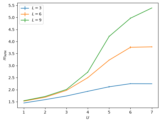

4.2.9Interpretation of the curves¶

An increase with $U$ indicates stronger antiferromagnetic correlations as double occupancy becomes energetically costly. A finite signal on a small lattice is expected even in the semimetal and is not by itself evidence of long-range order. Moreover, the raw structure factor grows with system size in an ordered state, so its square root cannot be compared directly as an intensive order parameter. Use the normalization given above before extrapolating $m_s$ towards $L\to\infty$ .

The transition discussed here is a zero-temperature quantum phase transition. In two dimensions, this spin-rotation-invariant model has no spontaneous Néel order at nonzero temperature in the thermodynamic limit. The present finite-size, finite-temperature curves therefore show correlations approaching the ground-state behaviour, not a sharp thermal transition. At large $U$ , the exchange scale $J=4t^2/U$ becomes small, so cooling relative to $J$ is especially important. Spin correlations diagnose the magnetic part of the transition; this notebook does not directly measure the charge gap.

Credits: João C. Inácio 2026

References¶

Gross, D. J., & Neveu, A. (1974). Dynamical symmetry breaking in asymptotically free field theories. Physical Review D, 10(10), 3235–3253. 10.1103/physrevd.10.3235
Wang, F.-H., Sun, F., He, C., & Xu, X. Y. (2026). Resolving Quantum Criticality in the Honeycomb Hubbard Model. arXiv. 10.48550/ARXIV.2602.03656
Li, T., Jiang, S., Li, L., Zhang, Y., Kang, K., Zhu, J., Watanabe, K., Taniguchi, T., Chowdhury, D., Fu, L., Shan, J., & Mak, K. F. (2021). Continuous Mott transition in semiconductor moiré superlattices. Nature, 597(7876), 350–354. 10.1038/s41586-021-03853-0
Xia, Y., Han, Z., Zhu, J., Zhang, Y., Knüppel, P., Watanabe, K., Taniguchi, T., Mak, K. F., & Shan, J. (2026). Bandwidth-tuned Mott transition and superconductivity in moiré WSe2. Nature, 650(8102), 585–591. 10.1038/s41586-025-10049-3
Yang, J., Chen, G., Han, T., Zhang, Q., Zhang, Y.-H., Jiang, L., Lyu, B., Li, H., Watanabe, K., Taniguchi, T., Shi, Z., Senthil, T., Zhang, Y., Wang, F., & Ju, L. (2022). Spectroscopy signatures of electron correlations in a trilayer graphene/hBN moiré superlattice. Science, 375(6586), 1295–1299. 10.1126/science.abg3036
Chang, X., Tao, Z., Shen, B., Tian, W., Hu, J., Pistunova, K., Watanabe, K., Taniguchi, T., Heinz, T. F., Li, T., Mak, K. F., Shan, J., & Jiang, S. (2026). Electric-Field-Tuned Consecutive Topological Phase Transitions between Distinct Correlated Insulators in Moiré <mml:math xmlns:mml=“http://www.w3.org/1998/Math/MathML” display=“inline”> <mml:mrow> <mml:msub> <mml:mrow> <mml:mi>MoTe</mml:mi> </mml:mrow> <mml:mrow> <mml:mn>2</mml:mn> </mml:mrow> </mml:msub> <mml:mo>/</mml:mo> <mml:msub> <mml:mrow> <mml:mi>WSe</mml:mi> </mml:mrow> <mml:mrow> <mml:mn>2</mml:mn> </mml:mrow> </mml:msub> </mml:mrow> </mml:math> Heterobilayer. Physical Review Letters, 136(9). 10.1103/gt9l-954n
Biedermann, J., & Janssen, L. (2025). Twist-tuned quantum criticality in moiré bilayer graphene. Physical Review B, 112(4). 10.1103/hj61-dw78
Hawashin, B., Scherer, M. M., & Janssen, L. (2025). Gross-Neveu-XY quantum criticality in moiré Dirac materials. Physical Review B, 111(20). 10.1103/physrevb.111.205129
Huang, C., Parthenios, N., Ulybyshev, M., Zhang, X., Assaad, F. F., Classen, L., & Meng, Z. Y. (2025). Angle-tuned Gross-Neveu quantum criticality in twisted bilayer graphene. Nature Communications, 16(1). 10.1038/s41467-025-62461-y
Biedermann, J., & Janssen, L. (2026). Dirac quantum criticality in twisted double bilayer transition metal dichalcogenides. Physical Review B, 113(24). 10.1103/lr2x-nnks

4.2 Semimetal-to-Mott-insulator transition