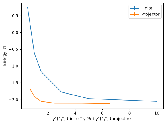
Comparison of finite temperature with projective algorithm

In this example we use the pyALF to read the simulation data of a 4-site ring from the previous run from disk and plot them together. For further details, see Sec. 2.3 of pyALF documentation.

1. Import Simulation class from the py_alf python module, which provides the interface with ALF, as well as numerical and plotting packages:

import matplotlib.pyplot as plt  # Plotting library

#
import numpy as np  # Numerical library
from py_alf import ALF_source, Simulation  # Interface with ALF
from py_alf.ana import load_res

alf_src = ALF_source(branch='main')    # Obtain ALF source code

Checking out branch main
Your branch is up to date with 'origin/main'.

Already on 'main'

2. Create instances of Simulation, specifying the necessary parameters, in particular the Projector to False for finite T and Projector to True for projector

# Finite T
sims_finite_T = []                                # Vector of Simulation instances
for beta in [0.5, 1, 1.5, 3, 5, 10]:               # Values of Beta
    sim = Simulation(
        alf_src,
        'Hubbard',                       # Hamiltonian
        {                                # Model and simulation parameters for each Simulation instance
        'Model': 'Hubbard',              #    Base model
        'Lattice_type': 'N_leg_ladder',  #    Lattice type
        'L1': 4,                         #    Lattice length in the first unit vector direction
        'L2': 1,                         #    Lattice length in the second unit vector direction
        'Checkerboard': False,           #    Whether checkerboard decomposition is used or not
        'Symm': True,                    #    Whether symmetrization takes place
        'Projector': False,               #    Whether to use the projective algorithm
        'ham_T': 1.0,                    #    Hopping parameter
        'ham_U': 4.0,                    #    Hubbard interaction
        'ham_Tperp': 0.0,                #    For bilayer systems
        'beta': beta,                     #    Inverse temperature
        'Ltau': 0,                       #    '1' for time-displaced Green functions; '0' otherwise
        'NSweep': 600,                   #    Number of sweeps per bin
        'NBin': 50,                      #    Number of bins
        'Dtau': 0.05,                    #    Ltrot=beta/Dtau
        'Mz': True,                      #    If true, sets the M_z-Hubbard model: Nf=2, N_sum=1,
        },                               #             HS field couples to z-component of magnetization
    )
    sims_finite_T.append(sim)

# Projector
beta = 0.5
sims_projector = []
for theta in [0.1, 0.25, 0.5, 1.0, 2.0, 3.0]:               # Values of Theta
    sim = Simulation(
        alf_src,
        'Hubbard',                       # Hamiltonian
        {                                # Model and simulation parameters for each Simulation instance
        'Model': 'Hubbard',              #    Base model
        'Lattice_type': 'N_leg_ladder',  #    Lattice type
        'L1': 4,                         #    Lattice length in the first unit vector direction
        'L2': 1,                         #    Lattice length in the second unit vector direction
        'Checkerboard': False,           #    Whether checkerboard decomposition is used or not
        'Symm': True,                    #    Whether symmetrization takes place
        'Projector': True,               #    Whether to use the projective algorithm
        'Theta': theta,                  #    Projector parameter
        'ham_T': 1.0,                    #    Hopping parameter
        'ham_U': 4.0,                    #    Hubbard interaction
        'ham_Tperp': 0.0,                #    For bilayer systems
        'beta': beta,                     #    Inverse temperature
        'Ltau': 0,                       #    '1' for time-displaced Green functions; '0' otherwise
        'NSweep': 600,                   #    Number of sweeps per bin
        'NBin': 50,                      #    Number of bins
        'Dtau': 0.05,                    #    Ltrot=beta/Dtau
        'Mz': True,                      #    If true, sets the M_z-Hubbard model: Nf=2, N_sum=1,
        },                               #             HS field couples to z-component of magnetization
    )
    sims_projector.append(sim)

3. Read the simulation data from disk

%%capture

sims_list = [sims_finite_T, sims_projector]
dict_list = ['beta', 'Theta']
ener_list = []
values_list = []

for i, sims in enumerate(sims_list):
    ener = np.empty((len(sims), 2))          # Matrix for storing energy values
    values = np.empty((len(sims),))          # Matrix for betas or theta values, for plotting

    for k, sim in enumerate(sims):
        dir = sim.sim_dir
        obs = load_res(dir)

        values[k] = sim.sim_dict[dict_list[i]] 
        ener[k] = obs.iloc[0][['Ener_scal0', 'Ener_scal0_err']]  # Store energy value

    values_list.append(values)
    ener_list.append(ener)

Where the cell magic %%capture suppresses the output of load_res(dir), which lists the data directories.

4. Plot the internal energies for finite T and projector

str_list = ['Finite T', 'Projector']

plt.xlabel(r'$\beta~[1/t]$ (finite T), $2\theta+\beta~[1/t]$ (projector)')
plt.ylabel(r'Energy$~[t]$')
for i in range(len(ener_list)):
    x = values_list[i] if i == 0 else 2 * values_list[i] + beta
    plt.errorbar(x, ener_list[i][:, 0], ener_list[i][:, 1], label=str_list[i])

plt.legend()
# plt.xlim(0, 2.02);

6.3 Comparison of finite temperature with projective algorithm