Testing against ED - Hubbard on a ring

In this example we use the pyALF interface to run ALF with the Mz choice of Hubbard-Stratonovich transformation on a four site ring, at $U/t=4$ and inverse temperature $\beta t = 2$ . For this set of parameters, the exact internal energy reads:

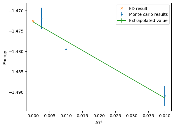
\left\langle -t \sum_{\langle i,j\rangle, \sigma} \hat{c}_{i,\sigma}^{\dagger} \hat{c}_{j,\sigma}^{\phantom\dagger} + U \sum_{i=1}^{N} \hat{n}_{i,\uparrow}\hat{n}_{j,\downarrow} \right\rangle = -1.47261997 t

(1)

To reproduce this result we will have to carry out a systematic $\Delta \tau t$ extrapolation keeping $\Delta \tau t L_\text{Trotter} = 2$ constant. Recall that the formulation of the auxiliary field QMC approach is based on the Trotter decomposition

e^{ -\Delta \tau \left( \hat{A} + \hat{B} \right) } = e^{ -\Delta \tau \hat{A}/2} e^{ -\Delta \tau \hat{B} } e^{ -\Delta \tau \hat{A}/2} + \mathcal{O} \left (\Delta \tau^3\right)

(2)

The overall error produced by this approximation is of the order $\Delta \tau^2$ .

Bellow we go through the steps for performing this extrapolation: setting the simulation parameters, running it and analyzing the data.

1. Import Simulation class from the py_alf python module, which provides the interface with ALF, as well as mathematics and plotting packages:

from py_alf import Simulation, ALF_source  # Interface with ALF
# 
import numpy as np                        # Numerical library
from scipy.optimize import curve_fit      # Numerical library
import matplotlib.pyplot as plt           # Plotting library
alf_src = ALF_source(branch='master')     # Obtain ALF source code

2. Create instances of Simulation, specifying the necessary parameters, in particular the different $\Delta \tau$ values:

sims = []                                # Vector of Simulation instances
print('dtau values used:')
for dtau in [0.05, 0.1, 0.2]:             # Values of dtau
    print(dtau)
    sim = Simulation(
        alf_src,
        'Hubbard',                       # Hamiltonian
        {                                 # Model and simulation parameters for each Simulation instance
            'Lattice_type': 'N_leg_ladder',  #    Lattice type
            'L1': 4,                         #    Lattice length in the first unit vector direction
            'L2': 1,                         #    Lattice length in the second unit vector direction
            'Checkerboard': False,           #    Whether checkerboard decomposition is used or not
            'Symm': True,                    #    Whether symmetrization takes place
            'ham_T': 1.0,                    #    Hopping parameter
            'ham_U': 4.0,                    #    Hubbard interaction
            'ham_Tperp': 0.0,                #    For bilayer systems
            'beta': 2.0,                     #    Inverse temperature
            'Ltau': 0,                       #    '1' for time-displaced Green functions; '0' otherwise
            'NSweep': 1000,                  #    Number of sweeps per bin
            'NBin': 100,                     #    Number of bins
            'Dtau': dtau,                    #    Only dtau varies between simulations, Ltrot=beta/Dtau
            'Mz': True,                      #    If true, sets the M_z-Hubbard model: Nf=2, N_sum=1,
        },                                    #             HS field couples to z-component of magnetization
    )
    sims.append(sim)

3. Compile ALF, downloading it first if not found locally. This may take a few minutes:

sims[0].compile()                        # Compilation needs to be performed only once

Checking out branch master
Your branch is up to date with 'origin/master'.

Already on 'master'

Compiling ALF... 
Cleaning up Prog/
Cleaning up Libraries/
Cleaning up Analysis/
Compiling Libraries

entanglement_mod.F90:35:2:

   35 | #warning "You are compiling entanglement without MPI. No Renyi entropy results possible, all other observables still work!"
      |  1~~~~~~
Warning: #warning "You are compiling entanglement without MPI. No Renyi entropy results possible, all other observables still work!" [-Wcpp]
ar: creating archive modules_90.a
ar: creating archive libqrref.a

Compiling Analysis
Compiling Program
Compiling program modules
Parsing Hamiltonian parameters
filenames: Hamiltonians/Hamiltonian_Kondo_smod.F90 Hamiltonians/Hamiltonian_Kondo_read_write_parameters.F90
filenames: Hamiltonians/Hamiltonian_Hubbard_smod.F90 Hamiltonians/Hamiltonian_Hubbard_read_write_parameters.F90
filenames: Hamiltonians/Hamiltonian_Hubbard_Plain_Vanilla_smod.F90 Hamiltonians/Hamiltonian_Hubbard_Plain_Vanilla_read_write_parameters.F90
filenames: Hamiltonians/Hamiltonian_tV_smod.F90 Hamiltonians/Hamiltonian_tV_read_write_parameters.F90
filenames: Hamiltonians/Hamiltonian_LRC_smod.F90 Hamiltonians/Hamiltonian_LRC_read_write_parameters.F90
filenames: Hamiltonians/Hamiltonian_Z2_Matter_smod.F90 Hamiltonians/Hamiltonian_Z2_Matter_read_write_parameters.F90
filenames: Hamiltonians/Hamiltonian_Spin_Peierls_smod.F90 Hamiltonians/Hamiltonian_Spin_Peierls_read_write_parameters.F90
Link program
Done.

4. Perform the simulations, as specified in each element of sim:

for i, sim in enumerate(sims):
    sim.run()                            # Perform the actual simulation in ALF

Prepare directory "/Users/fassaad/Programs/ALF/ALF_Tutorial/jupyterbook/source/05-caveats/ALF_data/Hubbard_N_leg_ladder_L1=4_L2=1_Checkerboard=False_Symm=True_T=1.0_U=4.0_Tperp=0.0_beta=2.0_Dtau=0.05_Mz=True" for Monte Carlo run.
Create new directory.
Run /Users/fassaad/Programs/ALF/ALF/Prog/ALF.out
 ALF Copyright (C) 2016 - 2022 The ALF project contributors
 This Program comes with ABSOLUTELY NO WARRANTY; for details see license.GPL
 This is free software, and you are welcome to redistribute it under certain conditions.
 No initial configuration

 Setting N_FL = 2 since this is mandatory for Mz-Hubbard model

Prepare directory "/Users/fassaad/Programs/ALF/ALF_Tutorial/jupyterbook/source/05-caveats/ALF_data/Hubbard_N_leg_ladder_L1=4_L2=1_Checkerboard=False_Symm=True_T=1.0_U=4.0_Tperp=0.0_beta=2.0_Dtau=0.1_Mz=True" for Monte Carlo run.
Create new directory.
Run /Users/fassaad/Programs/ALF/ALF/Prog/ALF.out
 ALF Copyright (C) 2016 - 2022 The ALF project contributors
 This Program comes with ABSOLUTELY NO WARRANTY; for details see license.GPL
 This is free software, and you are welcome to redistribute it under certain conditions.
 No initial configuration

 Setting N_FL = 2 since this is mandatory for Mz-Hubbard model

Prepare directory "/Users/fassaad/Programs/ALF/ALF_Tutorial/jupyterbook/source/05-caveats/ALF_data/Hubbard_N_leg_ladder_L1=4_L2=1_Checkerboard=False_Symm=True_T=1.0_U=4.0_Tperp=0.0_beta=2.0_Dtau=0.2_Mz=True" for Monte Carlo run.
Create new directory.
Run /Users/fassaad/Programs/ALF/ALF/Prog/ALF.out
 ALF Copyright (C) 2016 - 2022 The ALF project contributors
 This Program comes with ABSOLUTELY NO WARRANTY; for details see license.GPL
 This is free software, and you are welcome to redistribute it under certain conditions.
 No initial configuration

 Setting N_FL = 2 since this is mandatory for Mz-Hubbard model

5. Calculate the internal energies:

ener = np.empty((len(sims), 2))           # Matrix for storing energy values
dtaus = np.empty((len(sims),))            # Matrix for Dtau values, for plotting
for i, sim in enumerate(sims):
    print(sim.sim_dir)                    # Directory containing the simulation output
    sim.analysis()                        # Perform default analysis
    dtaus[i] = sim.sim_dict['Dtau']       # Store Dtau value
    obs = sim.get_obs()
    ener[i] = obs.iloc[0][['Ener_scal0', 'Ener_scal0_err']]  # Store energy value

/Users/fassaad/Programs/ALF/ALF_Tutorial/jupyterbook/source/05-caveats/ALF_data/Hubbard_N_leg_ladder_L1=4_L2=1_Checkerboard=False_Symm=True_T=1.0_U=4.0_Tperp=0.0_beta=2.0_Dtau=0.05_Mz=True
### Analyzing /Users/fassaad/Programs/ALF/ALF_Tutorial/jupyterbook/source/05-caveats/ALF_data/Hubbard_N_leg_ladder_L1=4_L2=1_Checkerboard=False_Symm=True_T=1.0_U=4.0_Tperp=0.0_beta=2.0_Dtau=0.05_Mz=True ###
/Users/fassaad/Programs/ALF/ALF_Tutorial/jupyterbook/source/05-caveats
Scalar observables:
Ener_scal
Kin_scal
Part_scal
Pot_scal
Histogram observables:
Equal time observables:
Den_eq
Green_eq
SpinT_eq
SpinXY_eq
SpinZ_eq
Time displaced observables:
/Users/fassaad/Programs/ALF/ALF_Tutorial/jupyterbook/source/05-caveats/ALF_data/Hubbard_N_leg_ladder_L1=4_L2=1_Checkerboard=False_Symm=True_T=1.0_U=4.0_Tperp=0.0_beta=2.0_Dtau=0.05_Mz=True
No orbital locations saved.
/Users/fassaad/Programs/ALF/ALF_Tutorial/jupyterbook/source/05-caveats/ALF_data/Hubbard_N_leg_ladder_L1=4_L2=1_Checkerboard=False_Symm=True_T=1.0_U=4.0_Tperp=0.0_beta=2.0_Dtau=0.1_Mz=True
### Analyzing /Users/fassaad/Programs/ALF/ALF_Tutorial/jupyterbook/source/05-caveats/ALF_data/Hubbard_N_leg_ladder_L1=4_L2=1_Checkerboard=False_Symm=True_T=1.0_U=4.0_Tperp=0.0_beta=2.0_Dtau=0.1_Mz=True ###
/Users/fassaad/Programs/ALF/ALF_Tutorial/jupyterbook/source/05-caveats
Scalar observables:
Ener_scal
Kin_scal
Part_scal
Pot_scal
Histogram observables:
Equal time observables:
Den_eq
Green_eq
SpinT_eq
SpinXY_eq
SpinZ_eq
Time displaced observables:
/Users/fassaad/Programs/ALF/ALF_Tutorial/jupyterbook/source/05-caveats/ALF_data/Hubbard_N_leg_ladder_L1=4_L2=1_Checkerboard=False_Symm=True_T=1.0_U=4.0_Tperp=0.0_beta=2.0_Dtau=0.1_Mz=True
No orbital locations saved.
/Users/fassaad/Programs/ALF/ALF_Tutorial/jupyterbook/source/05-caveats/ALF_data/Hubbard_N_leg_ladder_L1=4_L2=1_Checkerboard=False_Symm=True_T=1.0_U=4.0_Tperp=0.0_beta=2.0_Dtau=0.2_Mz=True
### Analyzing /Users/fassaad/Programs/ALF/ALF_Tutorial/jupyterbook/source/05-caveats/ALF_data/Hubbard_N_leg_ladder_L1=4_L2=1_Checkerboard=False_Symm=True_T=1.0_U=4.0_Tperp=0.0_beta=2.0_Dtau=0.2_Mz=True ###
/Users/fassaad/Programs/ALF/ALF_Tutorial/jupyterbook/source/05-caveats
Scalar observables:
Ener_scal
Kin_scal
Part_scal
Pot_scal
Histogram observables:
Equal time observables:
Den_eq
Green_eq
SpinT_eq
SpinXY_eq
SpinZ_eq
Time displaced observables:
/Users/fassaad/Programs/ALF/ALF_Tutorial/jupyterbook/source/05-caveats/ALF_data/Hubbard_N_leg_ladder_L1=4_L2=1_Checkerboard=False_Symm=True_T=1.0_U=4.0_Tperp=0.0_beta=2.0_Dtau=0.2_Mz=True
No orbital locations saved.

print('For Dtau values', dtaus, 'the measured energies are:\n', ener)

plt.figure()
plt.xlabel(r'$\Delta \tau^2$')
plt.ylabel('Energy')
plt.errorbar(dtaus**2, ener[:, 0], ener[:, 1], fmt='.', label="Monte carlo results")
plt.plot(0, -1.47261997, 'x', label='ED result')

def func(x, y0, a):
    return y0 + a*x**2
popt, pcov = curve_fit(func, dtaus, ener[:, 0], sigma=ener[:, 1], absolute_sigma=True)
perr = np.sqrt(np.diag(pcov))
xs = np.linspace(0., dtaus.max())
p = plt.plot(xs**2, func(xs, *popt))

plt.errorbar(0, popt[0], perr[0], label="Extrapolated value", color=p[0].get_color())
plt.legend()

5.2.1Exercises¶

Redo the extrapolation for different values of $\beta t$ (e.g., for $\beta t = 1$ , the internal energy is $-0.62186692t$ , and for $\beta t = 4$ , it is $-1.90837196t$ ).
Experiment with different settings for Checkerboard and Symm.

5.2 Testing against ED - Hubbard on a ring

5.2.1Exercises¶